How to see inside of your neural network: combining tensor histograms and Jacobian Sensitivity Analysis for quantized models

In this blog I will introduce a tool I have built for visualizing what’s happening inside neural networks in what I consider a useful way. It’s especially tailored towards quantized models, and will do two things: show you how the tensors in your model are distributed on the quantization grid, and, given some input to your model, show you how much each bin in your distribution contributes to the output of your model.
This blog will assume some understanding of neural networks, backpropagation, PyTorch, and quantization. If you’re new to quantization, I would highly recommend the Qualcomm quantization white paper, it’s a really, really good resource. With that context given, let’s get into it!
Neural networks are infamous for being black boxes. In training, you feed in data, and via backpropagation and some clever optimizers the model parameters learn to minimize the loss function. In inference, the model passes data through the layers, does some unseemly complicated transformations, and out comes some, hopefully desired, result.
This gets even worse when we quantize the model. Suddenly, both weight and activation tensors are getting rounded and clamped, gradients are going nuts, and making sense of what’s happening inside the model becomes that much harder. Maybe.
I have a background in quantization, and used to tear my hair out trying to understand what was going wrong when I quantized the model. I’ve since then built some tools for visualizing what happens inside of a neural network, especially a quantized neural network, and thought I would share them. I’ve personally found them useful, maybe you will too!
The technique I will outline does not require that models are quantized, but, weirdly, quantization actually makes it easier to code up, which is a really nice change from the usual quantization-is-painful coding aspect. For the rest of this blog I will assume we’re talking about a quantized model, but at the end I’ll discuss how this applies to a floating point model too.
The broad idea is to look at how your tensors lie on the quantization grid via a histogram, and then to look at how each much each histogram bin contributes to the final output of your model. That’ll tell you how the data looks in the forward pass, and what it’s final contribution ended up being to the output, all with respect to the quantization grid.
The reason quantization is relevant is because we can use the quantization grid as the basis for a histogram. We will use the quantization bins as a consistent basis for the histogram bins, e.g. 5 histogram bins per quantization bin, or 1 histogram bin per 3 quantization bins, or whatever. This histogram will capture the shape of the tensor in question, be it an activation or a weight tensor. This helps us visualize how the tensor maps onto the quantization grid, and that lets us know if our quantization grid is wack, or if our tensor could use some encouragement to take on a more-quantization friendly shape (e.g. entropy maximizing). But, we can do better.
Jacobian Sensitivity Analysis
IMO, the real magic is in incorporating Jacobian Sensitivity Analysis, which I will refer to as JSA.
A bit of a primer on JSA: it involves feeding data through the network, and then backpropagating the output, as is. We don’t use any fancy loss function, we just average the output of the model and backpropagate it. You just got out? Well tough, back in you go! If we just average the output, the resulting gradients represent the contribution of all of the model parameters and inputs to the output in question. Furthermore, by placing backwards hooks into a layer of the model to read the gradients passing through that layer you can see how much every element of its intermediary activation contributed to the final output.
Gradients can be a bit noisy, which can make JSA noisy. If analyzing a single input/output, you’d probably need to backpropagate a few noisy versions of it to get some reasonable, average signal in your JSA. But when JSA works, it’s really cool. It tells you how much each of your parameters are contributing to the output given the specific input you fed to the model, and can show you the same for the individual parts of the intermediary activations.
Tensor Histogram Implementation
Now, the nice thing is that we can combine the tensor histograms with JSA to get a nice visualization. Doing this is a little bit tricky, but the basic idea is that we generate the histogram in the forward pass, and get the gradients in the backward pass. I’ll just use the example of an activation since it’s a bit more complete. If we understand the activation example, then understanding the process for weights will be a piece of cake.
As we pass data through the model, for any arbitrary layer, we capture the intermediary forward activation with a pre-forward hook before the quantization step of the layer’s output, with the hook placed into the quantization module. As such, we are capturing the floating point tensor, just prior to it getting quantized, but we also have handy access to the quantization parameters of that tensor. The basic setup is depicted in the image below.

In our hook, we will calculate two things. The first is the histogram of the incoming data. For our histogram bin resolution, we can decide on something relative to the quantization grid, e.g. 5 histogram bins per quantization bin, and half of the histogram bins are placed inside of the quantization grid, which the other half split evenly outside the quantization grid. This former will ensure that we can see some of what’s happening inside the quantization bins (i.e. what the data looks like before getting rounded), and the latter helps us see what’s happening outside the quantization grid, e.g. how much of the tensor is getting clamped by quantization. Below is a snippet of the PyTorch code used inside the pre-forward hook, e.g. with HIST_MIN = HIST_MAX = 0.5 (how much we should extend the histogram bins beyond the edge of the quantization grid, in this case 50% on each side),HIST_QUANT_BIN_RATIO = 5 (5 histogram bins per quantization bin), module is equal to the quantization module i.e. requantization step, and local_input is equal to the incoming floating point tensor.
# Set min and max values for the histogram bins, given the quantization grid
hist_min_bin = (-HIST_XMIN * qrange - module.zero_point) * module.scale
hist_max_bin = (
    (HIST_XMAX + 1) * qrange - module.zero_point
) * module.scale

# If symmetric quantization, we offset the range by half.
if qscheme in (
    torch.per_channel_symmetric,
    torch.per_tensor_symmetric,
):
    hist_min_bin -= qrange / 2 * module.scale
    hist_max_bin -= qrange / 2 * module.scale

# Create the histogram bins, with `HIST_QUANT_BIN_RATIO` histogram bins per quantization bin.
hist_bins = (
    torch.arange(
        hist_min_bin.item(),
        hist_max_bin.item(),
        (module.scale / HIST_QUANT_BIN_RATIO).item(),
    )
    - (0.5 * module.scale / HIST_QUANT_BIN_RATIO).item()
    # NOTE: offset by half a quant bin fraction, so that quantization centroids
    # fall into the middle of a histogram bin.
)
tensor_histogram = torch.histogram(local_input, bins=hist_bins)

# Initialise stored histogram for this quant module
stored_histogram = dotdict() # a dictionary with dot-access notation
stored_histogram.hist = tensor_histogram.hist
stored_histogram.bin_edges = tensor_histogram.bin_edges
The second thing we will calculate is the mapping from each element of the tensor to the histogram bin. E.g., which bin did element [0,0,0,0] of the local_input tensor go into (with the assumption the tensor is 4D)? Which bin did element [0, 10, 20, 30] go in to? We need to store that mapping as well, below referred to as bin_indices. The bin_indices represents how each value of the activation got mapped to a histogram bin, and is basically a tensor of integers, with the same shape as the activation tensor, where the integers represent the bin the corresponding activation value was binned into.
# Create a map between the histogram and values by using torch.bucketize()
# The idea is to be able to map the gradients to the same histogram bins
bin_indices = torch.bucketize(local_input, tensor_histogram.bin_edges)

stored_histogram.bin_indices = bin_indices

# Store final dict in `act_histogram`, which is accessible outside the hook
act_histogram.data[name] = stored_histogram
It’s not shown in the above code to keep it simpler, but the histogram should accumulate values as more data is fed through the model, and the bin indices should always update. Here is the full code if you are interested. I am assuming we will do a backpropagation after every forward pass.
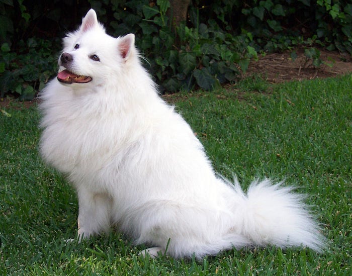
Below are the kind of plots we get for the activation of the last layer of a PTQ-observation quantized ResNet18 model when I feed an image of this dapper little Samoyed through the model:
In the histogram plot below, the blue represents the histogram of the activation. The grey lines represent the quantization centroids, and the red lines represent the edges of the floating point tensor. We can see the right red line extends beyond the grey zone, so we can derive that a little bit of the floating point tensor is getting clamped (everything between the right-red and the rightmost grey line).
In the top right, we have a subplot that shows the average behavior inside each quantization bin. We have 5 histogram bins per quantization bin, and that’s why we have 5 bars in the subplot. We see that the data is more or less uniformly distributed, which in my experience is typical for activations. However for weight tensors you can sometimes see twin-tower quantization issues, due to QAT (see this paper by Nagel et al. for a discussion of twin tower issues and how to overcome them). In the top right we also get some stats, e.g. 79% of the data is not in the bins that contain the quantization centroids, and some small fraction (0.04%) of the data is being clamped.

This is already quite useful, and a common visualization technique in quantization, e.g. see Figure 3 of this paper. We can see our quantization grid is reasonable, and that the data follows a normal-ish distribution.
Jacobian Sensitivity Analysis Implementation
Great, now we can do the JSA part. The idea is that we now add backwards hooks, and capture the gradients for the same layers we captured the forward histograms for. At this point, it may be useful to keep in mind that the gradient tensors have the exact same shape as the intermediary activation tensors, which makes sense as the gradients represent the contribution of each of the intermediary activation tensor values to the final output. The setup in the backwards pass looks like this:

One we’ve read the gradients with the backwards hook, we use the stored bin_indices to map the gradients to their respective histogram bins. To get the contribution of each histogram bin to the output, we sum up all of the gradients that were mapped to the same bin, for each bin, and take the absolute values. That will tell us how much each histogram bin contributed to the final output of the model, which I think is super cool!

Now, in one plot, we can see:
- Blue: How did the data interact with the quantization grid in the forward pass.
- Green: How much each histogram bin contributed to the output of the model.
These two tend to be correlated. If a lot of the activation “mass” is in a certain histogram bin, then that bin is probably going to have a disproportionate impact on the output. However, they’re not perfectly correlated, which I find really interesting. I think the JSA is a bit more informative than the forward pass, because it tells you, knowing all of the downstream effects of the network, what each bin actually contributed to the output. Here we can see that the negatively valued bins didn’t contribute basically at all to the final output where the model was classifying what the image represented. As far as our doggo protagonist is concerned, we could have saved quantization space by not assigning quantization range to any of the negative values of the tensor.
What about weight tensors?
The exact same holds true for weights, except we don’t need to capture any forward activations. We can just read the weight tensors as they are. However, for the JSA, we do still need to feed data through the model and backpropagate it. Fortunately, we don’t need to any of this fancy hook business. We can just backpropagate and read the gradients of off the weight tensor, e.g. module.weight.grad in PyTorch. Similarly to the activations, its easiest to place our data in the context of the quantization module so we can 1) see how the tensor quantizes, and 2) have a nice built-in grid we can use as the basis for our histogram bins.

Similarly to the activations, we can see that the distribution of the weight tensor, and what ends up actually being important for this output, are not the same. The “importance” has a noticeable dip near 0, and wider tails.
Generalizing to floating point models
There’s no reason this technique requires a fake-quantized model, it’s just convenient to leverage a quantization grid. People put a lot of effort into finding good quantization grids for tensors, and its easy to build off of all of that work, as it conveniently gives us a grid for each tensor.
But in principle, this can be applied to fully floating point models. If that’s what you would like to do, from a coding perspective I’d still recommend quantizing your model using some technique that doesn’t impact the model weights and only updates the qparams, e.g. PTQ observation (I have a follow-along coding tutorial available here for PTQ observation quantization if you’re curious), and just turn fake quantization off when generating these plots. That way you get the grid, without any of the influence of quantization operations. The quantization grid would only be used as the basis for the histogram bins, i.e. a plotting device.
The End + Other Resources
That’s it! You made it to the end!
I built this tool to solve my own problems, but hopefully you will also find it useful. I tend to use it for seeing if my quantization grids make sense, and gain some insight into what the data and weights in my model are really up to.
I have a Jupyter notebook available with all of the code in this blog running through an example, that goes way more into detail on a coding from how to use this tool. If you can forgive the plug, it’s part of an EasyQuant Github quantization repo that I’m working on. EasyQuant is going to be a bunch of quantization visualization tools, some improved quantization modules (faster, more versatile and scalable than PyTorch’s native quantization modules), a large suite of PTQ observers, off-the-shelf unit tests, tutorials, etc. Basically, all the stuff I wish I had when I got started in quantization, so I’ll be building that out. Feel free to contribute or use for your own projects!
I also have a video where I go over this tool, but it’s less detailed than this blog or the notebook: https://youtu.be/xozKHHFrpbY
But yeah that’s it, I hope you found this useful and/or interesting! Please leave a clap thingy, or a star on the repo. If you want to learn more about quantization, I have a YouTube channel where I do a lot of coding and theory tutorials on quantization. If you’re a complete beginner to quantization, again I can’t recommend the Qualcomm quantization white paper strongly enough.
Have a good one!